Image Detection via Vector Search

My friend and I are working on a project that involves fine-tuning a Stable Diffusion model. The goal is to generate consistent, functional 2-D video-game assets for rapid prototyping during development. To that end, we've been collecting image data for training, progress has been slow and the results weren't amazing because the main issue is our crawling strategy--it's is ass, that plus the fact we need to gather very specific asset images for our dataset.

Stable Diffusion is a text-to-image generator that can turn a prompt into a picture. Fine-tuning is the process of teaching that generator new concepts. To fine-tune a model, you need several thousand ideal images it hasn't seen before.

We figured we could improve our dataset by detecting--with reasonable confidence--whether an image is an asset worth training on. So we set up an image-detection system that uses image embeddings from a multimodal embedding model + vector database for similarity lookups. After building a reference collection of about 200 images we liked, we had a reliable way to boost dataset quality by making it easier to find good images.

A vector database indexes those high-dimensional vectors and lets you query them fast.

A multimodal embedding model ingests different data types--images, text, audio--and returns a single vector
(1 024 floats in our case). If we index these vectors in a vector-search database similar objects will be closer together in that vector space.

The pipeline is compact--under 100 lines of Python--even though it leans on both an embedding model and a vector database. I'll highlight the general-purpose approach so you can reuse it elsewhere. Whenever you have complex structured data to compare, pairing an embedding model with a vector database lets you ask, "Are these two things similar?" I'm using images today, but think broadly: fraud detection, product recommendations, whatever.

We built this on Atlas because SQL has caused us all enough pain. Sure, relational databases work great on paper--and in practice--but only if you've got actual time to model your data or tune your queries -- oh wait you work for an infinite-growth hyperscale company (or worse, a siloed mega-corp bound by five layers of regulation). MongoDB is not immune to those same problems, but it is more modern and in my opinion, easy to use. If you enjoy slapping an ORM on top of your data model and doing sixty-four joins just to fetch one record, be my guest. For everyone else, Atlas ships with Full-Text Search and Vector Search for free-ninety-nine.

The major caveat worth mentioning now is Atlas Vector Search lives in its own server process mongot--not inside the traditional mongod binary. Inserts hit the primary node first and only replicate via Change Stream to mongot. This means, sometimes you have to wait a bit before your data is searchable via the $search or $vectorSearch operators. Give it a bit (usually seconds, occasionally a coffee break) before you fire off that " find similar " query, or you'll likely receive an empty response.

With that out of the way, lets review the process from 30,000 feet:

1. Embed the data
2. Store the data
3. Query the data

That's really it--sort of. There are more steps, of course, but that's the big picture. By embedding and storing the data, we create a discrete feature space from which we can draw insights. In this case, the feature space contains vectors that describe an image and its properties. Given such a space, we can run calculations to see how similar a given set of embeddings is to the rest of the data.

I'm going to prove it to you--the best I can, my goal is to be an approachable technical writer can go into reasonable depth on the topic I'm presenting.

Extracting the Meaning from Images

I've selected four images--one cat, two dogs, and a nuclear reactor. Looking back, these in sequence might imply... never mind, moving on!

We're going to use an embedding model to generate a vector for each image, then run two functions: one for euclidean distance--how far apart two items are--and one for cosine similarity the dot product of the two vectors. A larger distance means the items are distinct, while a higher similarity means they’re, well, similar.

I want to demonstrate why this works with a practical example, enter the proof-of-proof-of-concept.

40-ish Lines to Prove the Proof-of-Concept's Concept

The snippet below embeds four image files, then pits them against each other using our Euclidean-distance and cosine-similarity helpers. Before executing the code, or scrolling further, do a quick gut check:

• Look at the pics up top and predict the scores.
• Will dogs and cats huddle together in vector space, or keep their distance?
• What happens when you throw a nuclear reactor into the mix--sky-high distance, near-zero similarity?
• Jot down your guesses, then see what happens.

from transformers import CLIPProcessor, CLIPModel
from PIL import Image
import torch, numpy as np
from pathlib import Path
from itertools import combinations

# Pick CPU if CUDA isn't available
device = torch.device("cuda" if torch.cuda.is_available() else "cpu")

# 0. Load the CLIP vision encoder & its processor
CKPT = "openai/clip-vit-base-patch32"  # 512-dim ViT-B/32 encoder
processor = CLIPProcessor.from_pretrained(CKPT)
vision    = CLIPModel.from_pretrained(CKPT).to(device).eval()

# 1. Four example assets; swap filenames or add more as you like.
img_dir = Path("examples")
files = {
    "cat": "cat.png",
    "dog A": "dog1.png",
    "dog B": "dog2.png",
    "reactor": "reactor.png",
}

# 2. Embed the data – use the CLS token (pooler_output)
vecs = {}
for label, fname in files.items():
    img = Image.open(img_dir / fname).convert("RGB")
    inputs = processor(images=img, return_tensors="pt").to(device)
    with torch.no_grad():
        out = vision.get_image_features(**inputs)
    vecs[label] = torch.nn.functional.normalize(out, dim=-1)[0].cpu().numpy()

# 3. Distance/Similarity helpers
def euclidean(a, b):
    a, b = np.asarray(a), np.asarray(b)
    return np.linalg.norm(a - b)

def cosine_sim(a, b):
    a, b = np.asarray(a), np.asarray(b)
    return float(np.dot(a, b) / (np.linalg.norm(a) * np.linalg.norm(b)))

# 4. Compare everything
print("pair".ljust(18), "euclidean".rjust(10), "cosine_sim".rjust(12))
print("-" * 42)

for (name_a, vec_a), (name_b, vec_b) in combinations(vecs.items(), 2):
    print(
        f"{name_a} vs {name_b}".ljust(18),
        f"{euclidean(vec_a, vec_b):9.2f}",
        f"{cosine_sim(vec_a, vec_b):11.2f}",
    )

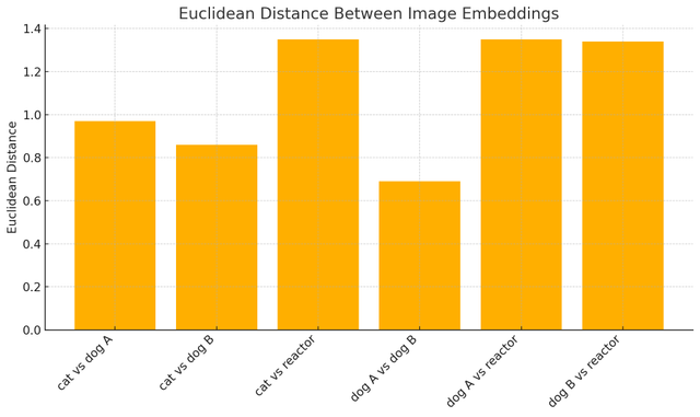
Running the code produced some output which I've charted below.

        pair                euclidean
-------------------------------------
cat vs dog A            0.97        
cat vs dog B            0.86        
cat vs reactor          1.35        
dog A vs dog B          0.69        
dog A vs reactor        1.35        
dog B vs reactor        1.34        

Euclidean distance values for each comparison

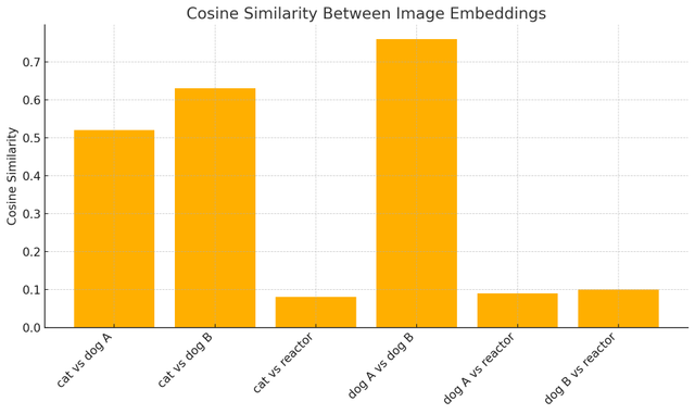
pair                cosine_sim
-----------------------------
cat vs dog A            0.52        
cat vs dog B            0.63        
cat vs reactor          0.08        
dog A vs dog B          0.76        
dog A vs reactor        0.09        
dog B vs reactor        0.10        

Cosine similarity values for each comparison

Dogs and cats appear to be more similar than either is to the nuclear reactor--nice.

It also looks like two similar pictures of dogs behave intuitively in terms of similarity and distance.

Hopefully this is helping to build your intuitive sense of how vectors created via embedding models can capture the "essence" of an object--in this case, an image despite being a list of seemingly random floating point values.

Okay, Detour Over--Back to Image Detection

Now that we understand how these vectors represent data in a discrete way--and how standard formulas help us use that--we can dive into the practical example. Zooming back out, this time to 20,000 feet, here are the next steps:

1. Create a vector-search index in Atlas to represent our data.
2. Collect reference images that match the type of data you care about.
3. Embed and write those reference images to your transactional database nodes.
4. Let those changes propagate to the Vector Search index.
5. Query the index via similarity searches to see whether an image resembles your reference data.

{
  "fields": [
    {
      "path": "embedding",
      "type": "vector",
      "numDimensions": 512,
      "similarity": "cosine"
    }
  ]
}

Demo Quickstart

Here are the files you'll need to get the environment setup and run the demo.

• pyproject.toml

• vector-detection-demo.py

• Golden Set

• Negative Set

• Test Image for find_similar

1. Create folders for the golden_set and negative_set and populate them with images, then download both the .toml and .py file.

2. uv sync

3. uv run python vector-detection-demo.py

"""
vector-detection-demo.py  – embed ➜ store ➜ search via Vector Search (HF Transformers)
"""

import glob, os, datetime as dt
from pathlib import Path

from dotenv import load_dotenv
from PIL import Image
import torch, pymongo
from transformers import CLIPProcessor, CLIPModel
from pymongo.collection import Collection
from bson.binary import Binary, BinaryVectorDtype  # PyMongo ≥ 4.11

load_dotenv()

# ─────────────────── Atlas / Collection setup ────────────────────
MONGODB_URI = os.getenv("MONGODB_URI")
MONGODB_DB = os.getenv("MONGODB_DB", "detection_demo")
COLL_NAME = os.getenv("REFERENCE_COLLECTION", "image_detection")
INDEX_NAME = os.getenv("VECTOR_INDEX_NAME", "image_detection_index")

# ─────────────────── Model & Processor  ───────────────────────────
device = torch.device("cuda" if torch.cuda.is_available() else "cpu")

# CLIP vision encoder (ViT-B/32) → 512-dim CLS vector
CKPT = os.getenv("CLIP_CHECKPOINT", "openai/clip-vit-base-patch32")
processor = CLIPProcessor.from_pretrained(CKPT, use_fast=False)
vision    = CLIPModel.from_pretrained(CKPT).to(device).eval()

DIMENSIONS = vision.config.vision_config.hidden_size  # 512 for CLIP base
as_bson = lambda v: Binary.from_vector(v, BinaryVectorDtype.FLOAT32)

mdb = pymongo.MongoClient(MONGODB_URI)[MONGODB_DB]
if COLL_NAME not in mdb.list_collection_names():
    mdb.command("create", COLL_NAME)
coll: Collection = mdb[COLL_NAME]

# Ensure Atlas Vector Search index exists
if not any(ix["name"] == INDEX_NAME for ix in coll.list_search_indexes()):
    coll.create_search_index(
        {
            "name": INDEX_NAME,
            "type": "vectorSearch",
            "definition": {
                "fields": [
                    {"path": "embedding", "type": "vector", "numDimensions": DIMENSIONS, "similarity": "cosine"}
                ]
            },
        }
    )


def embed_image(path: str):
    img = Image.open(path).convert("RGB")
    inputs = processor(images=img, return_tensors="pt").to(device)
    with torch.no_grad():
        out = vision.get_image_features(**inputs)
    return torch.nn.functional.normalize(out, dim=-1)[0].cpu().numpy()


def ingest_dir(folder: str, label: str):
    for fp in sorted(glob.glob(f"{folder}/*.[pj][np]g")):
        fname = Path(fp).name
        if coll.count_documents({"filename": fname}):
            continue
        vec = embed_image(fp)
        coll.insert_one(
            {
                "filename": fname,
                "filepath": str(Path(fp).resolve()),
                "embedding": as_bson(vec),
                "created_at": dt.datetime.utcnow(),
                "label": label,
            }
        )


def find_similar(img_path: str, k: int = 3):
    q_vec = embed_image(img_path)
    hits = coll.aggregate(
        [
            {
                "$vectorSearch": {
                    "index": INDEX_NAME,
                    "path": "embedding",
                    "queryVector": as_bson(q_vec),
                    "numCandidates": 5,
                    "limit": k,
                }
            },
            {"$project": {"_id": 0, "filename": 1, "label": 1, "score": {"$meta": "vectorSearchScore"}}},
        ]
    )
    print(f"\nTop-{k} matches for {Path(img_path).name}")
    for h in hits:
        print(f"{h['score']:.3f}  {h['label']:<12}  {h['filename']}")


if __name__ == "__main__":
    ingest_dir("golden_set", "marijuana")
    ingest_dir("negative_set", "plant/flower")
    find_similar("mimosa.png")

Code Walkthrough

I'm going to explain more interesting parts of the script above for those who are looking to learn how the code works. Starting with the following lines:

device = torch.device("cuda" if torch.cuda.is_available() else "cpu")

# CLIP vision encoder (ViT-B/32) → 512-dim CLS vector
CKPT = os.getenv("CLIP_CHECKPOINT", "openai/clip-vit-base-patch32")
processor = CLIPProcessor.from_pretrained(CKPT)
vision    = CLIPModel.from_pretrained(CKPT).to(device).eval()

The first line selects your GPU (if available). The next three load Hugging Face's CLIP vision stack in one go:

We embed an image like this:

img = Image.open(path).convert("RGB")
inputs = processor(images=img, return_tensors="pt").to(device)
with torch.no_grad():
    out = vision.get_image_features(**inputs)
    cls_vec = torch.nn.functional.normalize(out, dim=-1)[0]

torch.no_grad() is a context manager that allows us to use the model to retrieve the image embeddings without storing any calculated values for backpropagation. grad in this case is short for gradient computation; the same gradient descent algorithms which power neural network training. By disabling gradient computation, we save memory and computation time since we're only doing inference, not training.

1. processor(images=img, return_tensors="pt").to(device) applies the exact same transforms the model was trained with (resize → centre-crop → normalise → convert to tensor).
2. vision.get_image_features(**inputs) is the work-horse; it gives us a pure image embedding.Because we call get_image_features we get a pure image embedding. No captions, prompts, or file-name text are involved, so our similarity search depends solely on visual content.

The NumPy vector is then serialised with:

as_bson = lambda v: Binary.from_vector(v, BinaryVectorDtype.FLOAT32)

Which allows us to store our array of 512 floating point numbers into a compressed binary format, reducing on-disk index size.

Finding similar images

find_similar() repeats the same embedding step for an arbitrary query image, but instead of writing it to the database we feed the vector straight into the $vectorSearch aggregation stage. Atlas returns the top-k most similar documents, each with a similarity score from 0 to 1. Finding your ideal similarity threshold is a matter of evaluating the queries you run manually. This process can be automated, and I mean for instance you could simply prompt an agent to write out an evaluation script, there's not really an excuse for stuff like that anymore.

With these three moving parts—embed ➜ store ➜ search—you now have a complete, production-grade image-detection pipeline that clocks in at under 100 lines of Python.

Okay let's freaking run it alreadyYYYY

uv run vector-detection-demo.py

🔍  Top-3 for mimosa.png - This is a strain of weed with purple tones
0.967  marijuana  granddaddy_purple.png
0.967  marijuana  sour_diesel.jpg
0.965  marijuana  lemon_cherry_gelato.png

🔍  Top-3 for marigold.png - Marigolds are yellow flowers
0.859  plant/flower  silver_cocks_comb.png
0.857  plant/flower  celosia_caracas.png
0.848  plant/flower  damiana.png

🔍  Top-3 for dog1.png - This is a dog

So I passed in a picture of another cannabis bud, not currently in the reference set, a picture of a marigold to see if it would match against marijuana objects in the database. I guess unsurprisingly it matched the other flowers and things I had chosen for the negative set images. The picture of the dog well, it doesnt even pass the threshold for being a flower. Which now is probabaly a good time to clarify, picking negative images can be as impactful as picking positive ones.

I mean, maybe you're crawling a website that only has pictures of dogs, flowers, and marijuana, but you only want one of them -- the example is silly but you get the point. If you know exactly what you don't want you can apply the same pattern but inverse. Having both allows you to do interesting things, like running a simple majority vote across the labels of your k nearest neighbours to decide what an unknown image most likely is.

anyhoo, I've rambled enough, if you made it this far you're a real one! Thanks for sticking around, you win a good song recommendation!